Renaming A Column In Power Query Based On Position

The easiest way to rename a column in Power Query is to do it the same way you do in Excel - just double-click it and rename it. Sometimes though the column you are renaming can have different names with each refresh, so this method won’t work. We can use a List in Power Query to make this dynamic. Consider this very simple example:

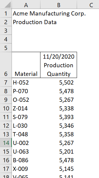
You receive this file every day, and the column name starting in Row 6, Column B, constantly changes. We are going to extract that date and make it a column, as it should be, and then rename both columns regardless of what they are called.

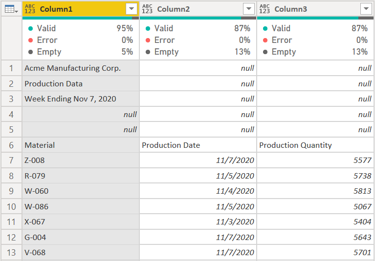
The first thing we do after importing the Excel file into Power Query is to remove the first 5 rows. Use the Remove Rows button on the Home ribbon, and remove the top 5 rows. If your data has rows that move around a bit because someone inserts or deletes rows above it, see this blog post on how to dynamically find that first row and remove the appropriate number of rows. Now we have something that looks like this:

Ok, let’s get to work. NOTE: If you had any “Changed Type” step created by Power Query, delete it. That will cause problems in the refresh. We’ll add it back at the end when our column names are predictable.

1) We need that date in a new Date column so we can relate it to a Date table later. If you have a date in your date model, you always need a good date table.

2) On the Add Column ribbon click Add Custom Column. Name the column “Date” and use this formula:

try 
    Date.FromText(
        Text.BeforeDelimiter([Column2], " ")
        )
otherwise null

You don’t have to have the line breaks and indents, it just makes it easier to read. Let’s break this down from the inside out:

• Text.BeforeDelimiter([Column2], “ “) - in the first row of data, this will return the “11/20/2020” text. In all other rows it will return errors, because there is no spaces in the other rows, and those are numbers, so there is no text to extract. That isn’t a problem and you’ll see why in a minute.

• Date.FromText() will take the date in the first row and convert “11/20/2020” to a real date. In all other rows, it returns errors.

• The try/otherwise construct says “Try this formula. If it works, give me the result. Otherwise, return null.” It is like IFERROR() in Excel. This is why the errors don’t matter. The try/otherwise construct takes care of it.

Now our data looks like this:

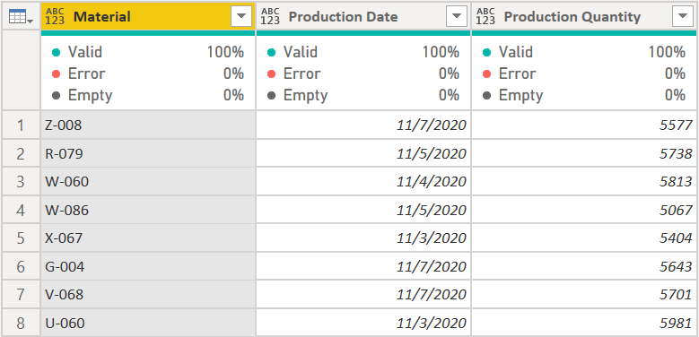
3) Right-click on the Date column and select the Fill menu, then Down. Now the date will fill the column.

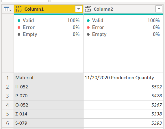
4) On the Home ribbon, click Use First Row as Headers. Again, remove any automatically added “Changed Type” step if Power Query added one. Now we have this:

Both the 2nd and 3rd column need to be renamed, and we cannot double-click to rename, otherwise the refresh will fail tomorrow when the date changes to Nov 21, 2020. If you did double-click though, this would be the formula Power Query would generate:

= Table.RenameColumns(
    #"Promoted Headers",
    {
        {"11/20/2020 Production Quantity", "Production Quantity"},
        {"11/20/2020", "Date"}
    }
)

We need to replace the first part of the renaming list (the list is in the curly brackets). We can use a function called Table.ColumnNames() for this. To see how it works, remove your manual renaming step, and type in this formula, and you will get the list shown below. It is each column name in the table from the Promoted Headers step.

= Table.ColumnNames(#"Promoted Headers")

To use this we need to get the column names from the 2nd and 3rd row. To get items from a list, you can refer to the index of an item in the list using curly brackets again, so change your formula to this, and you’ll get the column name shown below.

= Table.ColumnNames(#"Promoted Headers"){1}

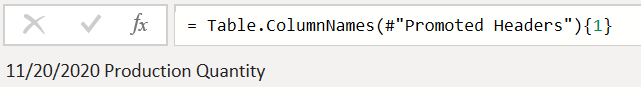
You’ll notice I used {1} to get the second item in the list. Power Query indexes at zero, so {0} would return the first item. Now you see where this is going?

5) Delete any steps you have up to the Promote Headers. Once again, manually rename the headers. This is so Power Query will generate the Table.RenameColumns() step for us and we will make minor tweaks. It should be this again:

= Table.RenameColumns(
    #"Promoted Headers",
    {
        {"11/20/2020 Production Quantity", "Production Quantity"},
        {"11/20/2020", "Date"}
    }
)

6) Replace the “11/20/2020 Production Quantity" with Table.ColumnNames(#"Promoted Headers"){1} and replace “11/20/2020” with Table.ColumnNames(#"Promoted Headers"){2}. It should now look like this:

= Table.RenameColumns(
    #"Promoted Headers",
    {
      {Table.ColumnNames(#"Promoted Headers"){1}, "Production Quantity"},
      {Table.ColumnNames(#"Promoted Headers"){2}, "Date"}
     }
)

It is dynamically finding the column name of the 2nd and 3rd columns and replacing it with specific text!

As always, set the data types for all columns at this point too now that we know what our column names will be.

Use List.PositionOf() To Find The First Row of Data In An Excel File

Excel can be one of the worst data sources for Power BI. Its greatest strength for users is also its greatest weakness for Power BI developers getting data out of it via Power Query - it is almost unlimited in its flexibility. So end users will do things that cause your refreshes to fail. Things like inserting columns, rows, merging cells, etc. I’m going to show you how to find data in a spreadsheet when users add or remove rows above the table you need. Consider the spreadsheet data below:

This is a simple grid of data. Ideally this would be in an Excel table, but often a Power BI developer cannot control how the data comes in, and most users still do not use Excel tables. So I call this a grid of data. And the problem with a grid of data is when it moves and you use Power Query to get the data, it will be missing information. For example, when you bring this Excel file into Power Query, it looks like this:

Fixing this is simple:

1. On the Home ribbon in Power Query, select Remove Rows, then Remove Top Rows, then type in the number 5.

2. On the Home ribbon, select “Use first row as headers”

Now it looks like this:

Perfect! We have good data. Next week, however, the user accumulating the production data add a few rows at the top of the file to include some notes about one of the facilities being down for maintenance one of the days.

Now the grid of data starts on row 8, not row 6 like before. When Power Query does the refresh, you get this:

Now you have a mess. the column names will load into Power BI as Column1, Column2, and Column3 if it loads at all. More likely you’ll just get a refresh error. If you had changed the data types (as you should) it would have broken right off of the bat when it tried to change the “Material” column to text. The Material column no longer exists! It is just Column1. The Production Date column is worse as if you tried to change that to a Date data type, that itself will generate errors because there is text in that column. In other words, this is a total mess. You could edit your Power Query code to skip the first 7 rows instead of the first 5, but that just becomes a cat and mouse game when the users adds or removes rows again in the future.

The better solution is to dynamically find the first row of data. Power Query has a function that will help with this. It is called List.PositionOf(). Basically what it does is it takes a list and tell you what position your search item is on in the list. Let’s walk through it with our new production data with the extra rows.

First, delete the Promoted Headers and Removed Top rows steps you created earlier so we are back to the below image. If there are any Changed Type steps, get rid of those as well. You should only have the Source and Navigation steps in the Applied Steps at the right side of the Power Query window.

We want to find the word “Material” here. Right-Click on the “Navigation Step” in the Applied Steps pane and click Insert After. It will create a Custom1 step that will simply have this in the formula bar: = Sheet1_Sheet - which is just pointing to the Navigation step. Change that to this:

= Sheet1_Sheet[Column1]

We told it to only show us [Column1] from the Sheet1_Sheet step. Sheet1_Sheet is just the name of the table. Confusingly Power Query hides this in the Navigation step. Here we can clearly see it. Note: If you are using this technique at any time after the Navigation step, the table name is just the name of the Applied Step. For example, if you had selected the first three columns and then selected Remove Other Columns from the ribbon, your step would be “Remove Other Columns” and the table name is #”Remove Other Columns” - the # and quotes are necessary if any table name has spaces in it.

Most Applied Steps in Power Query are just tables. But this one is not. You’ll notice after adding [Column1] after it, the name of the first column, it is now a list.

Now we are getting somewhere. Time to use List.PositionOf. Edit the formula above to this, and you’ll get the following screen.

= List.PositionOf(Sheet1_Sheet[Column1], "Material")

It found the word “Material” on row 7. Wait a minute… on the image above with the list, it shows Material on row 8. Power Query indexes at 0, so the first row isn’t 1, but 0. So Material is in position 7 in the list. This actually helps us with the next step.

Right-click on the Custom1 step and rename it something useful, like PositionOfMaterial. I recommend you use no spaces for this step. It makes referencing it later easier.

Right-click on PositionOfMaterial again and Insert Step After. Now, we need to get our original table and skip the first 7 rows, right? When you use the Remove Top Rows feature, Power Query creates a step using the Table.Skip function. We are going to do that manually. In the formula bar, you probably see =PositionOfMaterial and it still show the value. Get rid of that and type this:

= Table.Skip(Sheet1_Sheet, PositionOfMaterial)

Remember, our original table was Sheet1_Sheet. Table.Skip has this syntax: Table.Skip(TableName, RowsToSkip). TableName is Sheet1_Sheet in this case, and instead of hardcoding the RowsToSkip, we are using a variable, our PositionOfMaterial step. Now our data looks like this:

Now you can promote the first row as headers, change your data types, and continue on. Next week when our production supervisor turns in the report, it won’t matter if Material on on row 1 or 100, List.PositionOf() will find it for us and dynamically set the top of the table. Even if all of the header is deleted, List.PositionOf() will return 0 for the position of Material, and Table.Skip will effectively do nothing, skipping 0 rows. So it will still work for us.

This method will work with any kind of data, but Excel is the most common use for it. Most other data sources, like databases, SharePoint Lists, true Excel tables, and even CSV files, don’t have data moving up and down on you.